Combine Plots into a Single Grid

Communicating results in graphical format is a very common task in research. During my career, I can’t tell you how many times I’d have several Excel graphs that I rearranged in PowerPoint, to create a single grid layout to save as a png file for presentation in a manuscript. Every time you wanted to change a small feature in the figure, it resulted in extra work. That all changed when I started to use R for all of my research needs.

In R, grid is the major package used to align multple graphical objects, also called grobs, into a single layout. Using ggplot2, gtable, grid, and gridExtra, you can create grahpics of the highest quality. There are many features availble to provide exquisite control over creating complex graphs that you routinely find in the highest ranked journals, such as Nature.

In the future, I’ll add more content to this post to include many other features. Here, however, I demonstrate how to make a basic layout for six graphs in a single grid.

Layout Strategy

First, decide the layout strategy that you want to use. Visualize the layout in blocks, and then imagine the grids in terms of rows and columns. Once determined, the layout object essentially defines what plots reside in what columns and rows of the layout.

Checkout this video on Instagram for an example (don’t forget to like, follow, and subscribe!!)

Example layout:

color_fills <- c("gray", "green", "purple", "orange", "red", "black")

gs <- lapply(1:6, function(ii) grobTree(rectGrob(gp = gpar(fill = color_fills[ii],
    alpha = 0.5)), textGrob(paste("Plot", ii, collapse = " "))))

lay <- rbind(c(1, 1, 1, 2, 2, 2, 4, 4, 4), c(1, 1, 1, 2, 2, 2, 4, 4, 4), c(1, 1,
    1, 2, 2, 2, 5, 5, 5), c(3, 3, 3, 3, 3, 3, 5, 5, 5), c(3, 3, 3, 3, 3, 3, 6, 6,
    6), c(3, 3, 3, 3, 3, 3, 6, 6, 6))

top_title = textGrob("Example Layout", gp = gpar(fontface = "bold", col = "red"))

bottom_title = textGrob("Example Layout", gp = gpar(fontface = "italic", fontfamily = "Arial",
    col = "blue"))

right_title = textGrob("Example Layout", gp = gpar(col = "green", lty = "solid",
    fontsize = 16), rot = -90)

grid.arrange(grobs = gs, layout_matrix = lay, top = top_title, bottom = bottom_title,
    left = "Example Layout", right = right_title)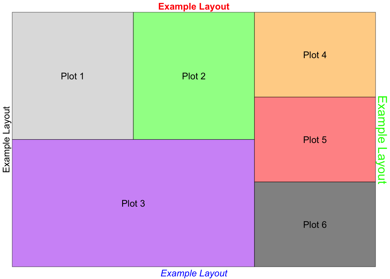

Note the example code to manipulate textGrob in the top, bottom, right, and left title positions. There are many other ways to manipulate text and add tables to the grid also.

Create Plots and Covert to Grobs

Here, I use the mtcars dataset to demonstrate how to create and layout the plots. Using ggplot2 create the plots of interest. Since the general features and layouts are perserved for each chart, ensure you are placing a chart in an appropriate layout grid. For example, if your grob is essentially a rectangle, don’t force it into a square layout. Also, work with the ggplot2 theme for appropriate display in the grid layout.

data("mtcars")

# Consider the axis and place the right data in the right shapes

p1 <- qplot(mpg, data = mtcars) + ggtitle("Distribution of MPG")

p2 <- qplot(mpg, data = mtcars, geom = "dotplot")

# you can use facet to plot multiple plots into a single plot prior to
# gird.arrange
p3 <- p1 + facet_wrap(~am, nrow = 1) + theme(legend.position = "none") + ggtitle("Transmission (0 = automatic, 1 = manual)")

# Simple x, y plots work well in square layouts
p4 <- qplot(mpg, wt, data = mtcars, color = cyl)

p5 <- qplot(mpg, disp, data = mtcars, color = cyl)

p6 <- qplot(mpg, hp, data = mtcars, color = cyl)

# Convert plots to grobs
g1 <- ggplotGrob(p1)
g2 <- ggplotGrob(p2)
g3 <- ggplotGrob(p3)
g4 <- ggplotGrob(p4)
g5 <- ggplotGrob(p5)
g6 <- ggplotGrob(p6)

grid.arrange function

Finally, use the grid.arrange function to combine the grobs into a single grid layout.

grid.arrange(g1, g2, g3, g4, g5, g6, layout_matrix = lay)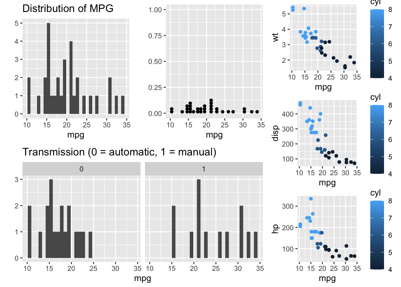

Until next time…