
Probability Distribution
Wow, more than a month passed since my last blog! I’ve been busy working on text mining and mapping free text to medical ontologies. The text mining utilizes heuristic and probabilistic approaches, so I decided to take a step back to review probability theory and distribution of probabilities. Below, I provide a list of discrete and continuous probability functions with links to R documentation, and look at few probability distributions (normal, geometric, and binomial). As time passes, I plan to revisit this blog to go more in-depth with the other probability distributions.
Quick Review of Probability:
- Probability theory is the study of random phenomena and their mathematical models. To review some of the basic concepts, I used “Probability and Mathematical Statistics” by Prasanna Sahoo (2013), which anyone can download.
- I thought it was well written, concise, and easy to follow. A good 20-page ‘Cliffs Notes’ type review can be found here.
## Warning in readPNG("/Users/jdstallings/Google Drive/Blog/dataindeed/static/
## images/cards.png"): libpng warning: iCCP: known incorrect sRGB profile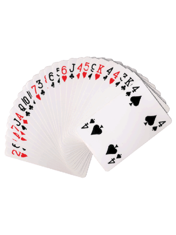
Probability
- In a deck of cards, all of the potential draws (i.e. 52 cards, also referred to as outcomes or events) constitute the sample space \(U =\{A_1,A_2,...A_{52}\}\).
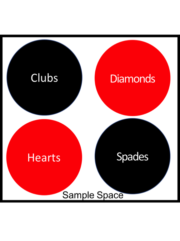
- Spades, \((A)\), constitute a subset of the sample space, \(A \subset U\). The probability of a given event, \(P\{A\}\), on the first draw dependents on the total events in \(N(A)\) and \(N(U)\).
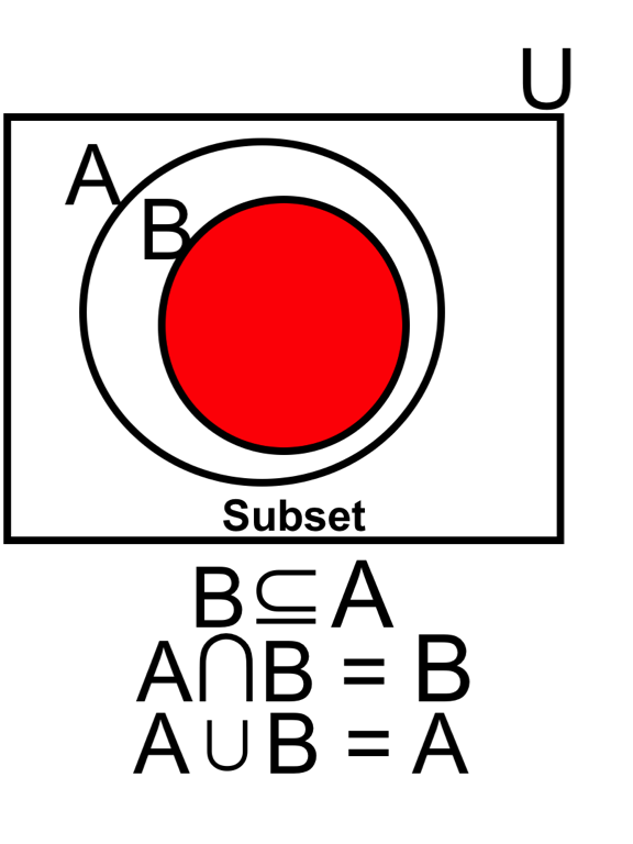
- Similarly, the Spade face cards \((B)\), i.e. Jack, Queen, and King of Spades, constitute a subset of Spades (A), \(B \subset A\). The probability of drawing a Spade is:
\[ \text{Eq1.} \quad P\{A\} = \frac{N(A)}{N(U)} = \frac{13}{52} = 0.25\]
- The probability of drawing a Spade on the first attempt will always lie between the probability of an impossible event (0), and a certain event (1):
\[ \text{Eq2.} \quad 0 \le P\{A\} \le 1\]
- for each event of A.
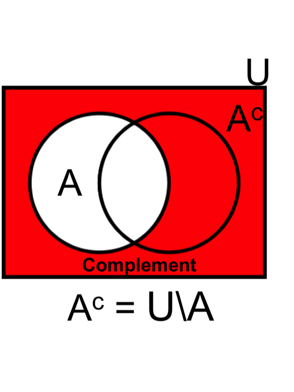
- The total sum of all probabilities in the sample space is equal to 1, \(P\{U\} = 1\). Therefore, the complement of the probability of drawing a spade is (i.e., drawing any other card in U), \(P\{A'\} = 1 - P\{A\} = 0.75\).
- The sum of an infinite number of probabilities in the following: \[ \text{Eq3.} \quad P \left\{ \bigcup_{i=1}^{\infty} A_i \right\} = \sum_{i=1}^{\infty} P\{A_i\}\]
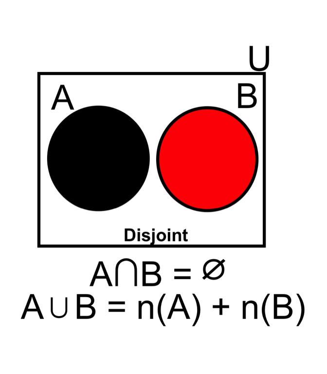
Disjoint Events
- Disjoint events (mutually exclusive events) do not occur at the same time. For example, the first and second trail when we drew from the deck are disjoint events (if we do not place the first card back into the deck).
- When considering disjointed events, the probability of the union of a finite number of mutually exclusive events are added: \[ \text{Eq4.} \quad P(A \cup B \cup C) = P(A) + P(B) + P(C)\]
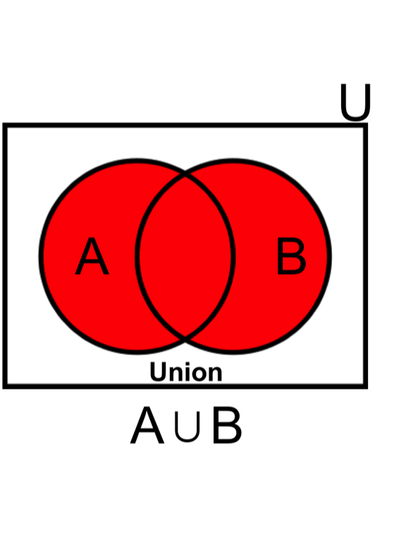
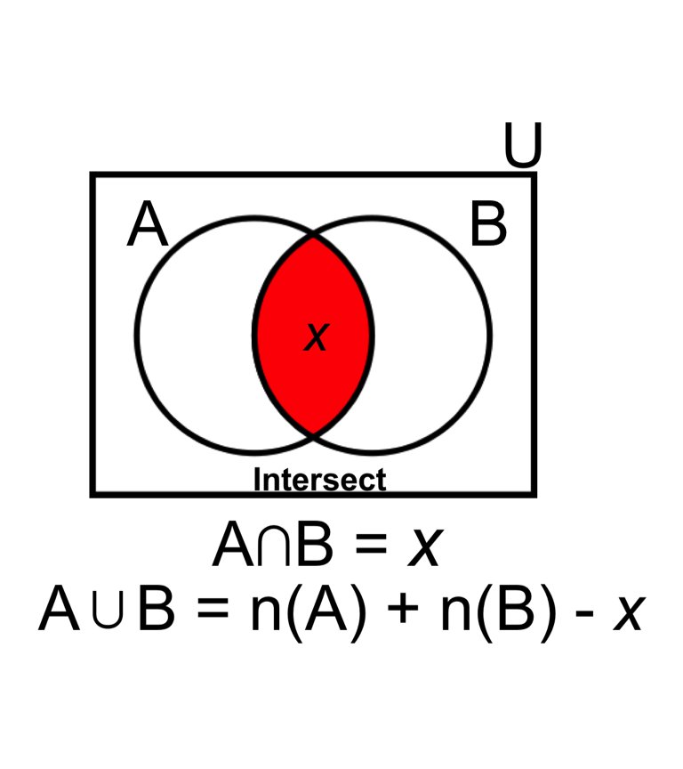
 - The probability of drawing a ‘Spade OR Ace’ includes areas of (A) plus (B) minus their intersect. For example:
\[ \text{Eq5.} \quad P(A \cup B) = P(A) + P(B) - P(A \cap B) = \frac{13}{52} + \frac{4}{52} - \frac{1}{52}= \frac{16}{52} = 0.308\]
- The probability of drawing a ‘Spade OR Ace’ includes areas of (A) plus (B) minus their intersect. For example:
\[ \text{Eq5.} \quad P(A \cup B) = P(A) + P(B) - P(A \cap B) = \frac{13}{52} + \frac{4}{52} - \frac{1}{52}= \frac{16}{52} = 0.308\]
Independence
- The probability of drawing a ‘Spade (A) AND Ace (B)’ in the first trial is determined by the multiplication rule because they are technically independent events.
- Independent events are unrelated and the outcome of one event does not impact the outcome of the other. The example of the ‘Spade (A) AND Ace (B)’ satisfies rule 1 below.
- When considering multiple draws (assuming the card from the first trial is returned to the deck), the probability of drawing a Spade and then a Club face card also satisfies the rule of independence. - If any of the following statements are true, then all three are true and the rule of independence is satisfied:
\[ \text{Eq6, Rule 1.} \quad P\{A \cap B\} = P(A) \times P(B)\]
- example: \[P(Spade \cap Ace) = \frac{13}{52} \times \frac{4}{52} = \frac{1}{52} = 0.019\]
- example: \[P(Spade \cap Club) = \frac{13}{52} \times \frac{3}{52} = \frac{26}{52} = 0.014\] \[ \text{Eq7, Rule 2.} \quad P(A|B) = P(A)\] \[ \text{Eq8, Rule 3.} \quad P(B|A) = P(B)\]
Conditional Probability
- Conditional Probability is the probability of an event given that a second event has occurred. For example: P(A|B) is read as ‘Probability of A GIVEN B:’ \[ \text{Eq9.} \quad P(A|B) = \frac{P(A \cap B)}{P(B)}\]
- or ‘Probability of B GIVEN A:’ \[ \text{Eq10.} \quad P(B|A) = \frac{P(B \cap A)}{P(A)}\]
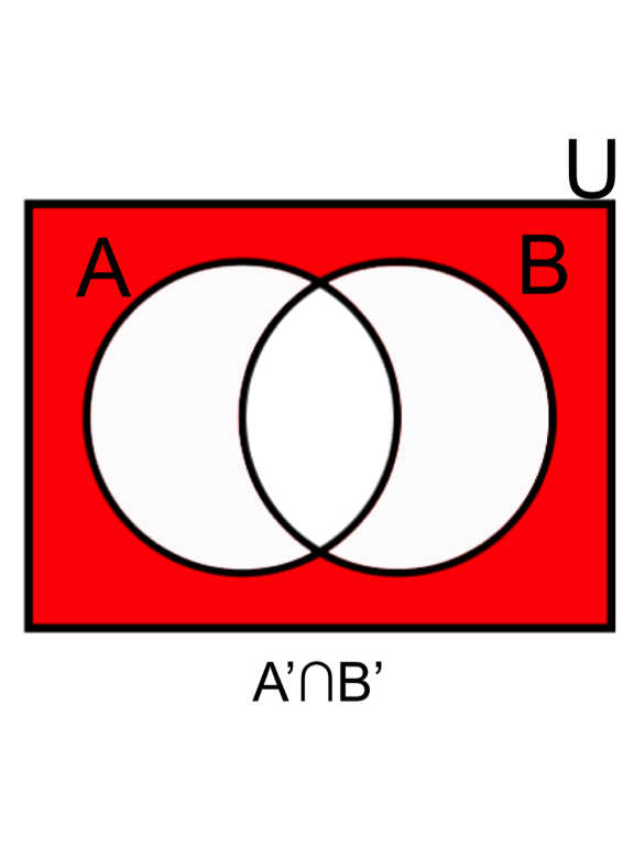
- Probability of a difference of two events: \[ \text{Eq11.} \quad P(A \cap B') = P(A) - P(A \cap B)\]
- DeMorgan’s law (1): the complement of the intersection of two sets is the same as the union of their complements.
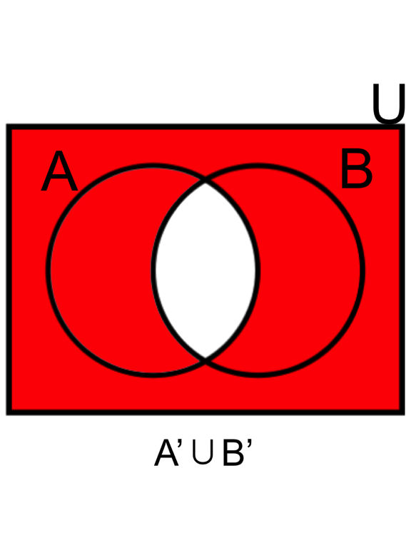 - DeMorgan’s law (2): the complement of the union of two sets is the same as the intersection of their complements.
 - The multiplication rule, permutation, and combination are the ways to count probabilities.
- Multiplication is straight forward, \(n_1 \times n_2\), as discussed above.
- Permutation focuses on the arrangement of objects with the order in which they are arranged, while Combination focuses on the selection of objects without regard to order. For example:
- Permutation:
\[ \text{Eq12.} \quad n(n-1)(n-2)...(n-r+1) = \frac{n!}{(n-r)!}= _n{P_r}\]
- Combination:
\[ \text{Eq13.} \quad \binom {n} {r} = \frac{n!}{(n-r)!r!}\]
Probability Distributions in R
- A probability distribution describes how the values of a random variable are distributed. For example, a series of coin tosses follows the binomial distribution, whereas height or weight measures randomly selected from a large data population is likely to follow a normal distribution. U
- Understanding probability distributions allow for statistical inferences on a specific number of coin tosses, or on the entire data population of height and weight measures as a whole.
This root for each function is prefixed by one of the letters:
p for "probability", the cumulative distribution function (c.d.f.) q for "quantile", the inverse c.d.f. d for "density", the density function (p.f. or p.d.f.) r for "random", a random variable having the specified distribution- For example, the normal distribution functions are pnorm, qnorm, dnorm, and rnorm. The binomial distribution functions are pbinom, qbinom, dbinom, and rbinom. And so forth.
For a continuous distribution “p” and “q” functions (c. d. f. and inverse c. d. f.) are useful to generate the distribution. For a discrete distribution, the “d” functions (p. f.) is useful.
Distribution: Correpsonding p, q, d, and r Functions.
Discrete Probability Distributions
Bernoulli: pbern, qbern, dbern, rbern. Unfortunately, you won’t find a discussion on Bernoulli distribution in any of the books in My Library. A Bernoulli trial is a random experiment with only two possible outcomes, usually viewed as “success” (\(p\)) or “failure” (\(1-p\)). A Bernoulli process is a series of Bernoulli trials, of which each trail is independent of the others. A Bernoulli distribution is the pair of probabilities of a Bernoulli event.
Binomial: pbinom, qbinom, dbinom, rbinom. The binomial distribution is obtained from the sum of independent Bernoulli random variables (i.e. heads/tails, success/failure). The distribution has two parameters: the number of repetitions of the experiment and the probability of success of an individual experiment.
\[ \text{Eq14.} \quad f(x) = \binom{n}{k} p^x (1-p)^{(n-x)} \text{ where } x = 0,1,2, \dots,n\]
x <- seq(1, 30, 1) # a sequence of 30 rolls
y <- dbinom(x, 30, prob = 1/2) # the distribution of probabilities

pbinom(26, 30, prob = 1/2) # cumulative probability at least 1 head in 30 flips
## [1] 0.9999958plot(x, y, type = "h", col = "red", lwd = 1.5,
xlab = "x",
ylab = "p(x)")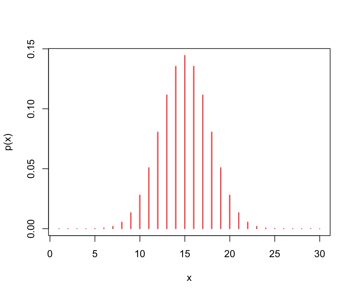
- Geometric: pgeom, qgeom, dgeom, rgeom. The geometric distribution probability is useful in modeling the number of failures before the first success in a series of independent trials. \[ \text{Eq15.} \quad P(n) = 1-p^n\]
x <- seq(1, 30, 1) # a sequence of 30 rolls
y <- dgeom(x - 1, prob = 1/6) # the distribution of probabilities

pgeom(x -1, prob = 1/6)[30] # probability on the 30th roll
## [1] 0.9957873plot(x, y, type = "h", col = "red", lwd = 1.5,
xlab = "Number of dice rolls it takes to sucessfully roll a 6",
ylab = "p(x)")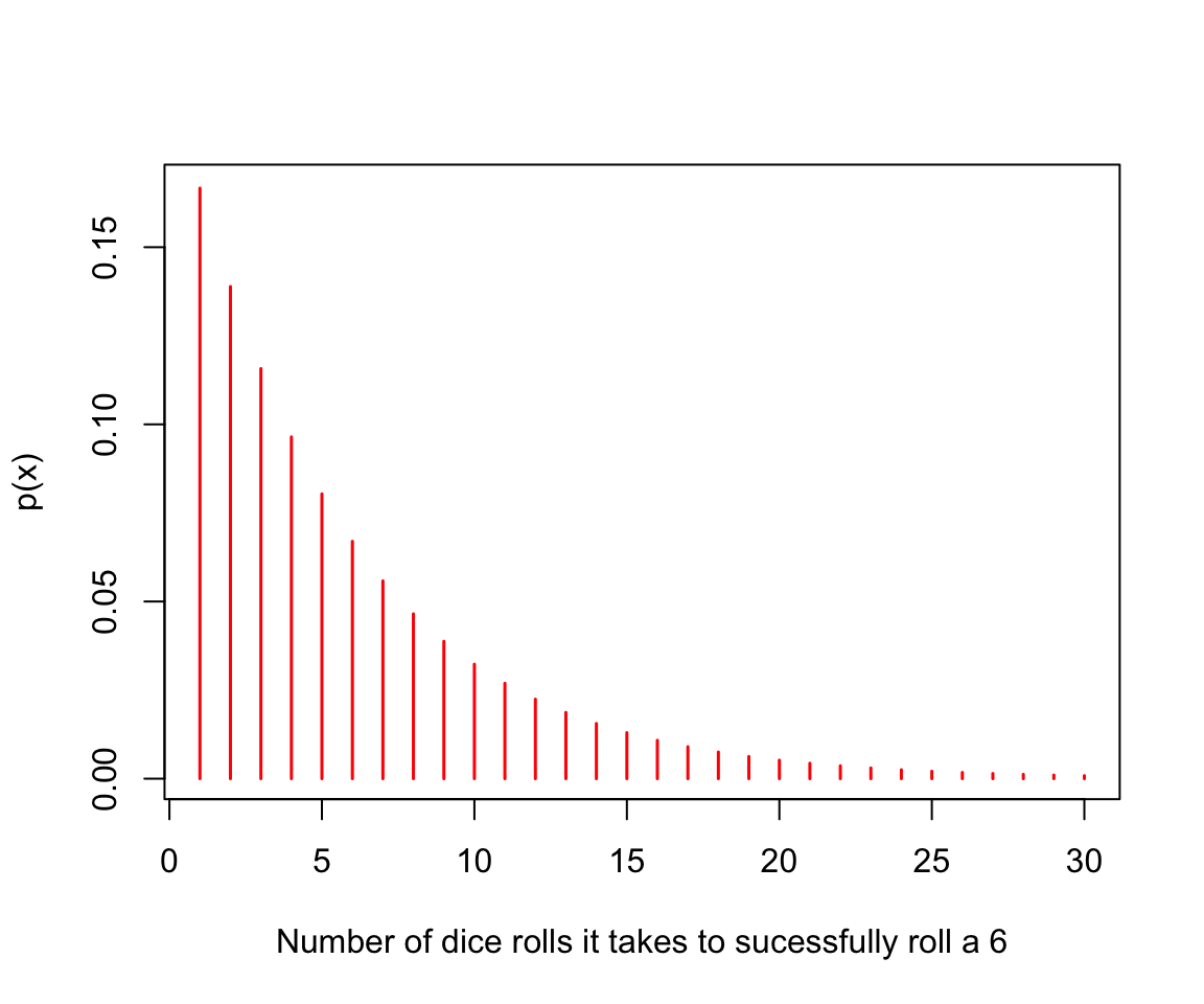
Hypergeometric: phyper, ghyper, dhyper, rhyper.
Negative Binomial: pnbinom, qnbinom, dnbinom, rnbinom.
Poisson: ppois, qpois, dpois, rpois.
Univariate continuous probability distributions
Beta: pbeta, qbeta, dbeta, rbeta.
Chi-Square: pchisq, qchisq, dchisq, rchisq. A random variable X has a Chi-square distribution if it can be written as a sum of squares:[eq1]where \(Y_{1}\), …, \(Y_{n}\) are mutually independent standard normal random variables. The importance of the Chi-square distribution stems from the fact that sums of this kind are encountered very often in statistics, especially in the estimation of variance and in hypothesis testing.
Exponential: pexp, qexp, dexp, rexp.
F: pf, qf, df, rf.
Gamma: pgamma, qgamma, dgamma, rgamma.
Normal: pnorm, qnorm, dnorm, rnorm. The normal distribution is often called Gaussian distribution, or “bell-shaped distribution.” The density of a normal distribution is symmetric around the mean. Deviations from the mean having the same magnitude and probability, but different signs. The further a value is from the center of the distribution, the less probable it is to observe that value.
- R’s equation for dnorm is the following:
\[ \text{Eq16.} \quad (x) = 1/(\sqrt{(2\pi)} \sigma) e^-((x - \mu)^2/(2 \sigma^2))\]
- where \(\mu\) is the mean of the distribution and the \(\sigma\) is standard deviation.
x <- seq(-20,20, by = .1) # the range of variables
y <- dnorm(x) # 401 random variables based on a normal distribution

dnorm(0, mean = 4,sd = 10) # calcualte the density if the mean and standard deviation are known
## [1] 0.03682701plot(x, y, type = "h", col = "red", lwd = 1.5,
xlab = "",
ylab = "p(x)")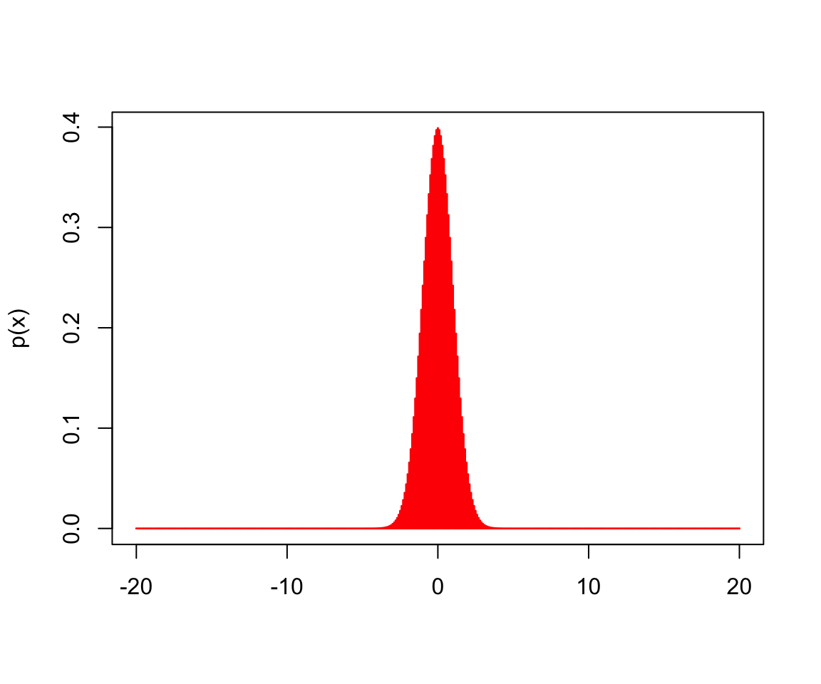
Multivariate probability distributions
Cauchy: pcauchy, qcauchy, dcauchy, rcauchy.
Logistic: plogis, qlogis, dlogis, rlogis.
Log Normal: plnorm, qlnorm, dlnorm, rlnorm.
Studentized Range (Tukey): ptukey, qtukey, dtukey, rtukey.
Weibull: pweibull, qweibull, dweibull, rweibull.
Wilcoxon Rank Sum Statistic: pwilcox, qwilcox, dwilcox, rwilcox.
Wilcoxon Signed Rank Statistic: psignrank, qsignrank, dsignrank, rsignrank.
Until next time…